Module 5. Sample size

General sampling considerations

Considerations for household-based surveys

Calculation of sample size for a single cross-sectional cluster survey

Calculation of sample sizes for baseline and follow-up cluster surveys

Subgroup comparisons and their effect on sample size

This module provides examples and information on sample size determination. It is essential that an experienced sampling statistician be included in the team to develop and implement the sampling plan, and to undertake quality control measures as the survey progresses.

General Sampling Considerations

The right sample size is crucial for meeting survey objectives and for calculating costs. Sample size calculations depend on a number of factors, and it is worth investing time to consider the advantages and disadvantages of different scenarios. Individuals with sampling expertise should either be part of the Technical committee or consulted to check that the proposed sample size will meet the survey’s objectives.

If the survey is intended to measure many indicators among different population groups, a choice must be made as to which indicator will drive the sample size. The major factors that influence sample size decisions are related to the survey purpose and design (see Module 4: Survey design), and include:

• stratification and proposed number of survey strata;
• key indicators, population groups of interest, and whether estimates are required at the stratum or national level;
• precision and level of statistical confidence required for the indicator of interest in the specific population group at the stratum and national levels; and
• available budget.

Each of these four factors will influence decisions about sample size in different ways.

1. Stratification and proposed number of survey strata

• The sample size calculation should initially be based on desired strata-level precision for the indicator and population group. The national sample size is the sum of the strata specific sample sizes.
• In some cases, stratified data are collected for certain indicators, while feasibility issues may mean that only national estimates, or estimates for more than one stratum combined, are collected for other indicators. Feasibility may be limited by the magnitude of the calculated sample size or by factors such as laboratory costs for analysing sufficient samples to obtain reliable estimates at the stratum level.

2. Key indicators, population groups of interest, and whether estimates are required at the stratum or national level

• In cases where the principal aim of the survey is to obtain stratified data for one key indicator, the survey sample size may be based on the calculated sample size for this indicator in the main population group of interest. For example, it may be decided that due to the implementation of an oil fortification programme, vitamin A deficiency is the driving micronutrient of interest. Sample size for this key indicator is then determined largely by:
  • the level of stratification
  • the desired precision for the estimate
  • the expected survey design effect on the indicator.
• If the survey objectives include more than one key indicator, or measurements of a key indicator in different population groups, the stratum-level sample size requirements should be calculated for each indicator for each population group separately. The resulting sample sizes should then be considered against the feasibility of obtaining these sample sizes at the stratum or national level. Box 5.1 presents an example of sample size calculations for several key indicators and for more than one population group of interest. It also includes discussion about the feasibility of obtaining estimates at the stratum and national levels.

3. Precision and level of statistical confidence around point estimates required for the indicator of interest in the specific population group at the stratum and national levels.

• The reason for including a specific indicator will help determine how precise or reliable the indicator measurement needs to be. For example, if a micronutrient indicator is being measured to obtain an initial estimate of the prevalence of deficiency, lower precision may be acceptable. If it is being measured to assess the impact of a targeted intervention, higher precision may be needed to assess the change in prevalence.
• A balance needs to be found between acceptable precision, logistics and cost. Box 5.1 includes discussion of this for the example presented. In general, micronutrient surveys are conducted to provide estimates with programmatically applicable precision, as opposed to research-level precision. For a stratified survey, having good precision at a sub-national level will lead to a more precise national estimate.
• The confidence level describes the confidence interval (CI) around the measurement derived from the survey. The CI is presented as a range of values within which the true value is likely to fall. A 95% CI is used as the standard in most surveys, and is used in the sample size calculations in this module. The width of the CI around the estimate, for example ± 0.05 (± 5%) or ± 0.10 (± 10%) is a measure of the level of precision. For example, if the prevalence of iron deficiency was estimated to be 40% among women of reproductive age, a precision of ±10% would provide 95% confidence limits that range between 30% and 50%. This means that one can state with 95% confidence that the prevalence in the population lies somewhere between 30% and 50%. Whether this is an acceptable level of precision depends on the expected use of the survey results.
• Precision is affected by a number of features, including the design effect for each indicator. Further information about precision and the design effect, as well as about how these are affected by the balance between number and size of clusters, is provided in later sections of this module.

Box 5.1. Sample size estimates for multiple indicators across a single stratum (based on household survey design)

Nutrition-related measure of interest	Indicator	Population group	Precision		Estimated prevalence (%) a	Estimated design effect b	Required sample size c	Number of individuals needed to achieve target sample size c	Number of households needed to obtain target sample size d
Stunting	Height/length	Children under 5 years	±	7	40	1.5	280	370	530
Anaemia	Haemoglobin	Children 6-59 months	±	10	45	2	190	235	430
Anaemia	Haemoglobin	Women 15-49 years	±	10	30	2	160	190	165
Iron Deficiency	Ferritin	Children 6-59 months	±	10	50	2	192	240	430
Iron Deficiency	Ferritin	Women 15-49 years	±	10	50	2	192	225	195
Household coverage of adequately iodized salt	Household salt iodine level	Household	±	10	60	3	280	300	300

^a An estimated prevalence of 50% will give the largest required sample size if all other factors remain the same. Therefore, for an indicator with no information on estimated prevalence, 50% is generally used to ensure an adequate sample size.

^b Design effect estimated based on previous surveys, estimates from other countries, and knowledge from the national (iodized) salt supply system.

^c The formulae used to calculate the (rounded) target sample size and number of individuals needed to achieve this sample size (accounting for expected response rates) are described in later sections of this module.

^d This column applies where the survey is designed based on a random selection of households from a complete household listing in each cluster, and takes into consideration the expected proportion of household members within each population group. However, not all surveys are designed in this way. In some cases, a census of households is conducted in advance, and then only households with, for example, children under 5 years of age are visited to obtain the required sample size for this population.

4. Available budget

• Sample size is the principal factor for the total cost of both fieldwork and sample analysis. Therefore, the sample design, sample size, and available budget need to be considered together.

The interplay between these factors and their effect on sample size is illustrated in Figure 5.1.

Other factors to consider in calculating a sample size include:

• Finite population correction (FPC) factor:
  • Most cluster survey sample size formulae assume an infinite or very large number of PSUs in the geographic area of interest. If the total number of PSUs is “small,” as may be the case in some Pacific Island nations, for example, a smaller sample size can be used by taking into consideration the FPC factor. There is no exact value for what makes a “small” target population, but in general the FPC factor is considered when the total number of PSUs from which the sample is selected is less than 1000. For geographic areas with at least 1000 PSUs, the FPC factor will not substantially change the sample size and is very rarely used.
• Response rate:
  • In calculating the sample size, an estimate of the response rate is needed, and the sample size needs to be increased to account for non-response. For household surveys that include individual-level indicators, there are two levels of response: the household-level response and, for participating households, the individual response.

Fig. 5.1. Factors affecting sample size

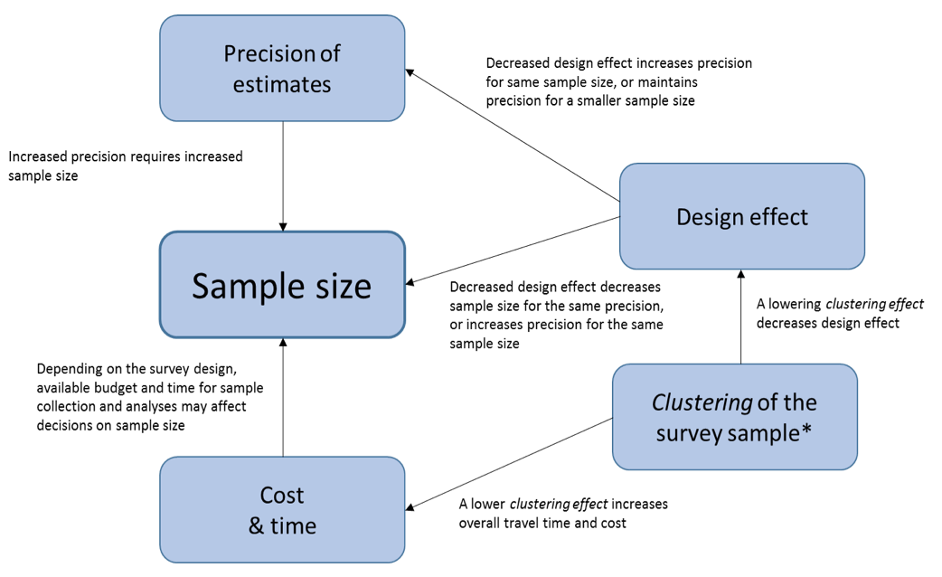*The clustering effect can be lowered by increasing the number of clusters and decreasing the number of samples per cluster. The concept of clustering effect is described in later sections of this module.

Considerations for household-based surveys

For individual-level indicators in a household-based survey where households are randomly selected from a complete listing of households in the cluster, the number of households to visit depends on:

• the number of individuals needed to obtain estimates with sufficient precision for the indicator within that population group;
• the average size of a household;
• the number of individuals from the population group of interest expected within each household; and
• the expected response rate.

More detail on how these factors are accounted for is described in Box 5.2.

The decision about selecting the survey sample from all households or from households that meet a specified criterion requires expert consultation to clearly understand the advantages and disadvantages of each approach and their effect on interpreting the resulting data.

If the number of survey households to include in the sample is based on the numbers required for preschool-age children, then it may not be necessary to collect data from all eligible WRA in the households. In such a case, it may be best to do a random selection of WRA. Possible methods include the random selection of one WRA per household, or selecting all WRA from every third household. The approach needs to be decided at the survey design stage and cannot be changed during the fieldwork. In all cases, it is important to document the total number of eligible individuals in each household, because this information will be needed to determine the sampling weight at the data management stage.

It is also important to keep in mind that not all information needs to be collected on every survey subject or household. For example, it may be reasonable to perform more expensive tests on a subsample of biological samples, such as every second survey participant within one population group, so long as minimum sample size requirements for that indicator are satisfied.

After making the initial calculations of sample sizes for the desired precision at the stratum level, decisions need to be made about feasibility. Where one population group (in this case children under 5 years of age) requires visiting significantly more households, then the following can be considered:

1) identifying in advance households with this population group and randomly selecting as many of these as are required to find 370 children (this would bias other indicators to be representative of households with children under 5).
2) accepting a reduced stratum level precision for estimates of 10% (stunting among children under 5), 11% (household coverage of adequately iodized salt), and 13% (anaemia and iron deficiency among children 6-59 months). (This would reduce the required number of households to approximately 250 per stratum).
3) it may be determined that reliable estimates for indicators among this group are only possible at the national level rather than at sub-national (e.g., stratum) levels.

Box 5.2. Household- versus individual-level indicators

For household-level indicators, the number of households to visit will be determined by the number of completed household interviews (and, where included, food tests or samples) required to obtain estimates with the desired precision, accounting for the expected number of occupied households and the response rate for interview and sample collection. For example, 95% of selected households may be occupied and have an adult household member willing to answer questions about the household, while food sample collection may only be feasible in a lower proportion due to non-availability of the food item and/or non-response for collection.

For individual-level indicators in a household-based survey with a random selection of households from a complete household listing, the number of households to visit depends on four factors:

1. the required sample size for the number of individuals within a specific population group
2. the average household size
3. the proportion of the population comprising the population group of interest
4. the expected household and individual response rates for population-group specific interviews and for sample collection.

Multiplying the average household size by the proportion of the population group of interest in the national population provides the average number of eligible individuals expected per household. The number of households that need to be visited to achieve the required sample size can then be calculated from this, taking into consideration the expected response rate.

The final number of households to be visited to obtain data for the required number of subjects from a specific population group may be calculated by dividing the sample size (in this case 766) by the product of: [the average household size (3.9) multiplied by the proportion of the specific population group in the population (0.31) multiplied by the expected response rate for households (90%) and individuals (85%)]. This must also take into account the design effect, DEFF, which is a measure of the homogeneity within a cluster and the variability between clusters.

As an example, where a survey sample size for non-pregnant women of reproductive age (WRA) in a geographic area has been determined to be 766 (already accounting for DEFF), the average household size is 3.9, the proportion of non-pregnant WRA in the population is 0.31, the household response rate is expected to be 0.9 (90%), and the individual response rate for consenting to biological sample collection is expected to be 0.85.

The number of this population group (WRA) per household would be expected to be 3.9 x 0.31 = 1.2. Therefore, the team can expect to obtain data from more than one eligible woman per household on average. However, the response rate also needs to be considered. The final number of households to visit to obtain information or samples from 766 WRA, based on the information above, could be calculated as:

Calculation of sample size for a single cross-sectional cluster survey

Because sample size calculations are based on a number of different decisions and estimates, a range of sample sizes may be produced for a single indicator and population group. The assumptions behind the differences between sample sizes should be discussed with the Steering committee and Technical committee. A rationale for acceptable precision and the final proposed size should be agreed for each indicator and population group. Whatever decisions are made regarding sample size calculations, they should all be documented in the methodology sections of the survey protocol, human subject documents and final survey report.

Box 5.3. Special considerations for calculation of sample size in surveys assessing iodine status

Current recommendations for survey sample collection and data analysis are based on the determination of population - not individual - iodine status. For example, a median urinary iodine concentration (UIC) of 100-199 µg/L indicates adequate iodine intake among a population of school-age children.¹

Iodine status is normally assessed in cluster surveys using casual (single sample) urine samples. Because there is high variability in individual iodine excretion throughout the day, a single urine sample and resulting UIC cannot be considered to reflect an individual’s iodine status. Therefore, it is not valid to calculate or present prevalence of iodine deficiency (which implies a count and comparison of people with adequate and inadequate iodine status).

According to the UNICEF 2018 guidance,2 there is uncertainty on the best methods for power calculations to determine population iodine status using spot UIC measurements. Therefore, programme managers may act conservatively and have sample sizes higher than required to determine population iodine status. For example, a common starting point is a 30-cluster survey with 30 urine specimens per cluster for nationally representative estimate. Any subnational stratification requires additional consideration, such as residence, region, socio-economic status, or level of salt iodization. Further, sample sizes need to be adjusted for expected DEFF and non-response. The UNICEF guidance points readers to technical documents for sample size calculations specific to urinary iodine.

Cluster survey sample size calculations start with the same calculation as would be used for a survey using the single random sampling (SRS) method. However, the calculation then takes into consideration the survey design, the expected proportion of the population group of interest within a household, and the expected response rates.

Step 1: Calculate the sample size using the SRS method

This calculation is based on the formula:

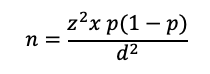
Where:

n is the calculated sample size

z is the statistic that defines the level of confidence required

p is an estimate of the key indicator to be measured by the survey in the population group of interest, for example, the prevalence of iron deficiency among WRA, expressed as a proportion of that population

d is the desired level of precision, or the margin of relative error to be obtained.

Generally, z = 1.96, which is the z-statistic for the 95% confidence level. If the expected estimate of the key indicator (p) is not known, the value of 0.5 (or 50%) is used because it produces the largest sample size (for a given value of d). If the proportion is expected to be between two values, select the value closest to 0.5. For example, if the proportion is thought to be between 0.65 and 0.75, use 0.65 for the sample size calculation.

Common values for d for national level estimates are usually around ±5% for indicators with estimated prevalence in the range of 20%–80% (for example, anaemia), and around ±3% for less common or very common events (for example, wasting, or household coverage of iodized salt). It is often acceptable to use a value of d higher than ±5% at a stratum level, with the knowledge that the precision around the national estimate will be narrower.

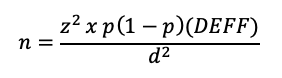
Step 2. Accounting for the Design Effect in Calculating Sample Sizes for Cluster Surveys

Cluster sampling is more feasible than SRS for large-scale surveys because it reduces the number of locations to visit and to map, and in which to set up field laboratories. However, cluster sampling introduces the “clustering effect”, which describes the fact that households in the same cluster tend to be more alike in terms of certain characteristics (for example, income, education and access to a fortified food product) than households across the general population. This clustering effect increases the variance between clusters so that it lowers the precision around an estimate that would have been found based on the same sample size calculated for SRS sampling. This change in precision due to clustering is described as the design effect (DEFF). The DEFF is a measure of the homogeneity within a cluster and the variability between clusters. It indicates how much larger the sampling variance (square of the standard error) is for the cluster sample compared to a simple random sample of the same size.

Unless the DEFF was calculated from previous survey data, it will need to be estimated at the stage of sample size calculation, based on prior field experience (unpublished data or subject matter expertise) or from published literature. Some indicators such as wasting (low weight-for-height) may have a small DEFF, while other indicators such as vitamin A capsule distribution may have a large DEFF. In rare cases, the DEFF may be less than 1, in which case a value of 1 should be used for sample size calculations. The DEFF is calculated using the intra-class correlation (ICC), which is a metric of the similarity of clusters in the outcome of interest. Box 5.4 provides more details on the ICC and how this affects the DEFF.

Calculation of sample size for a cluster survey incorporating the DEFF requires a modified version of the previous equation:

There are four important principles that can be applied to keep the DEFF (and sample size) as low as possible:

1. Use as many clusters as is feasible. For a non-stratified survey, the recommended minimum number is 30 clusters in the first stage of sampling. For a stratified survey, the recommended minimum is 25 per stratum. Up to a certain limit, the DEFF will continue to decrease as the number of clusters increases. Sampling more than 40 clusters per stratum does not provide much additional benefit to survey precision, in general.
2. Use the smallest cluster size (number of households per cluster) as is feasible, generally aiming for a minimum of 10 observations for each population group per cluster.
3. Use a constant cluster size.
4. Select a random sample of households at the final stage to increase geographic dispersion (see Module 7: Selecting households and participants).

Note: The DEFF (and hence the precision) for an indicator is affected by the number of observations per cluster, not the number of households visited. As an example, for a sample of 1200 households, a lower DEFF and higher precision would be achieved by selecting 40 clusters of 30 households each instead of 20 clusters of 60 households each.

Box 5.4. Relationship Between the Design Effect and the Intra-Cluster Correlation

The ICC is a measure of the degree of homogeneity (similarity with respect to the variable of interest) of the units (households or individuals) within a cluster. It is sometimes referred to as the “rate of homogeneity”, or ROH. Because units in the same cluster tend to be similar to one another in terms of income, climate/environmental conditions and attitudes, the ICC is almost always positive. The DEFF can be described in terms of the ICC and vice versa.

For a given deff and average number of units sampled per cluster (n̅), the ICCcan be estimated as:

If estimates of the ICC and average number of units per cluster are available, the DEFF can be calculated as:

The DEFF is significantly affected by the number of observations within one cluster. However, the relationship between the DEFF and the ICC means that the DEFF can be estimated for a subsequent survey that may have a different number of observations per cluster, using the equations above.

For example, analysis of data from the 2015-16 Malawi Micronutrient Status Survey found a DEFF of 1.9 for anaemia among children 6–59 months of age ¹. This estimate was based on 105 clusters with an average of 13.8 children per cluster (n=1452). If another survey was being planned with a design to select an average of 16 children per cluster, the ICC-DEFF relationship could be used to estimate the expected DEFF for this second survey.

The DEFF for the second survey with an average of 16 children per cluster would be estimated as:

Therefore, the estimated DEFF for anaemia for a survey with 16 children per cluster is 2.05, and this would be used in the sample size calculation.

¹ National Statistical Office, Community Health Sciences Unit [Malawi], US Centers for Disease Control and Prevention (CDC), Emory University. Malawi Micronutrient Survey 2015-16. Atlanta: US Centers for Disease Control and Prevention; 2017 (https://dhsprogram.com/pubs/pdf/FR319/FR319.m.final.pdf, accessed 20 June 2020).

Step 3: Accounting for Response Rates

Determining the sample size for household- and individual-level indicators must take into consideration the expected response rates of households and of individuals, and the availability of fortifiable foods. Box 5.2 describes factors to consider. Household and individual response rates can be estimated based on experience from previous similar surveys. Typically, response rates are higher for questionnaire-related indicators, such as an assessment of knowledge or behaviour, and they are lower for food sample collection (usually considered a household-level indicator) and for biological specimens, especially from young children or pregnant women. Ensuring community sensitization to the survey can greatly improve response rates, but when calculating the sample size, it is better to use a relatively conservative estimate.

Non-response can occur at different levels, for example the household interview, individual interview, and food sample and biological specimen collection. Here are potential reasons for non-response:

• None of the household members may be available during the time of the survey (the household is away on a temporary basis).
• The entire household may choose not to participate.
• Some individuals within a household may refuse to participate, may be sick, or may not be available during the survey.
• Some individuals may partially participate, such as agreeing to answer questions but refusing to provide a food sample or biological specimen collection.
• The fortifiable food of interest may not be available for collection within the household.
• The volume of blood or food sample collected may be insufficient for laboratory analysis.

All of these possible reasons for non-participation or non-response should be taken into consideration. The final number of households to be visited to obtain data for the required number of participants from a specific population group may be calculated as:

Where:

j is the expected response rate as a proportion (household response multiplied by individual response for interview/biological specimen collection)

k is the average household size

l is the proportion of the total population accounted for by the population group of interest

d is the desired level of precision, or the margin of relative error to be obtained

DEFF is the design effect

z is the statistical value derived from the normal distribution table for a given level of confidence (for example, z=2.58 when the type I error, or level of significance: alpha (α)=0.01).

An example calculation for one indicator is shown in Box 5.5.

The ”Survey sample size calculator” online tool can facilitate the process of sample size calculation and makes it easy to see, in the above equation, the effect of changing precision or other variables on final sample size. Additional computer-based programs to perform sample size calculations can be found at www.OpenEpi.com.

There may be differences between hand-calculated sample size estimates and computer-based calculations due to rounding and slight variations in sample size formulae, but these differences are usually minor.

Box 5.5. Example Sample Size Calculation

The required (unit) sample size to assess vitamin A deficiency among children 6–59 months of age was calculated assuming p = 0.35 (prevalence of deficiency 35%), level of acceptable precision d =.05 (or ±5%), and DEFF = 2.5:

Sample sizes are always rounded up, so this would be a desired sample size of 874 children.

The average household size is 3.9 and the proportion of this age group in the population is 0.09, while the household response rate is 90% and the individual response rate is 85%. In order to achieve the target sample size of 874 children, 3255 households should be visited.

Decreasing the acceptable level of precision by 2% reduces the number of households to visit by more than 1500. Using an acceptable precision of 0.07, or ±7%, results in a household sample size of 1661 households.

Depending on the setting, different precision values or different expected DEFF values may be appropriate. For example, an estimated household coverage of adequately iodized salt of 20% would indicate significant problems with implementing universal salt iodization. It could be decided that a precision of ±10% would be sufficient because the programme response would be the same whether the true prevalence was anywhere between 10% and 30%. On the other hand, if the prevalence of the indicator of interest is very low or very high, or expected to be close to the cutoff value for public health significance, it may be desirable to have a precision of ±5% or, in rare cases, an even higher precision of ±2.5%. However, the impact of such increased precision on sample size must be weighed against the programmatic application of the outcome.

Calculation of sample sizes for baseline and follow-up cluster surveys

Household surveys are frequently designed to estimate the prevalence of certain indicators and to assess changes in these indicators over time. Often, an initial survey serves as a baseline to identify the need for an intervention or to assess status before its implementation. A follow-up survey is then conducted to assess changes in selected indicators, and potentially to introduce additional indicators. The sample size for each survey should be estimated using survey design parameters that account for:

• assumptions about expected changes in the indicator estimates over a proposed time period and the reliability of the data to capture this change; and
• whether the same or different clusters and households will be included in the initial and follow-up surveys.

There are different methods to calculate the required sample size. One example is provided in the Feed the Future population-based survey sampling guide ¹ and calculator². You can also find details of the OpenEpi method at www.OpenEpi.com. To calculate the required sample size, the following estimates and assumptions are needed:

n is the calculated sample size.

DEFF is the estimated design effect (while the formula allows for one DEFF across the two surveys, it is recommended to use the larger DEFF for the sample size calculation)

Z is the statistic that defines the level of confidence required

α (“alpha”) is the desired level of two-sided significance of the difference in estimated proportions between surveys, usually 0.05 or 5% (corresponding to a 95% CI)

p is an estimate of the key indicator to be measured by the survey in the population group of interest, for example, the prevalence of iron deficiency among WRA, expressed as a proportion of that population

q_i is 1 − p_i

1 − β (the type II error) is the expected chance of detecting a difference between the two surveys, usually 0.8 (80%) or 0.9 (90%), also known as power

p₁ is the estimate of the key indicator to be measured in the population group of interest, for example, prevalence of anaemia or proportion of households using adequately iodized salt at the time of the baseline survey

q₁ is 1 − p₁

p₂ is the estimate of the key indicator to be measured in the population group of interest, expressed as a proportion, at the time of the follow-up survey

q₂ is 1 − p₂

In the formula below, it is assumed that the sample size in each of the two surveys will be the same. The formula is:

Where:

Table 5.1 and 5.2 display the different two-sided Z values (Z_α/2) that can be used for different significance levels and the one-sided Z values (Z_1-β) that can be used for various Power (1 − β) levels.

Table 5.1 Two-sided Z values for different significance levels

Significance level (α)	Two-sided Z value
0.01	2.576
0.05a	1.960
0.10	1.645

^a Value used in example.

Table 5.2 Two-sided Z values for different significance levels

β value	Power (1 − β)	One-sided Z value
0.01	.99	−2.326
0.05	.95	-1.645
0.10	.90	-1.282
0.20a	.80	-0.842

^a Value used in example.

An example of a calculation is shown in Box 5.6. It is important to remember that a higher power and lower significance level will increase the needed sample size

Once the baseline survey has been completed, the components assumed for the sample size calculation for the baseline (namely prevalence at baseline, DEFF, response rates and accuracy of projected estimates) for the follow-up survey should be revised based on the known information from the baseline survey.

You can find additional help in comparing the sample sizes of a baseline and a follow-up survey using the “Survey sample size calculator” online tool.

Box 5.6 Example Sample Size Calculation for Baseline and Comparative Follow-Up Surveys

A country is going to begin fortifying flour with iron. The survey team estimates that the baseline prevalence of anaemia is 50% among WRA, and expects that iron fortification of flour will lower the anaemia prevalence in this group to 40% over 12 months.

Example of sample size calculation for those that wish to calculate this by hand:

p₁ (proportion of anemia in the selected population group at baseline) = 0.50, q₁ = 0.50

p₂ (proportion of anemia in the selected population group at follow-up after intervention) = 0.40,

q₂ = 0.60

α = 0.05, therefore Z_(α/2) = 1.96

β = .20, therefore Z_(1-β) = -.842

DEFF = 2

Assuming equal sample sizes, p is calculated as:

In this example, the sample size would be 776 individuals in each cross-sectional survey, that is, 776 for the baseline survey and 776 in the follow-up survey. The number of households to visit to obtain information from 776 individuals would depend on the expected response rate and the proportion of the population group in each household.

Subgroup comparisons and their effect on sample size

The discussion of factors affecting sample size is based on surveys designed to obtain national and subnational estimates for the prevalence of certain nutrient-related indicators. However, sometimes an objective of the survey will be to compare subgroups, such as comparing males to females, or comparing the prevalence of a specific deficiency among a defined population group in households that do not use a fortified food to the equivalent estimate in households that do. If these types of comparison are important, then the sample size will usually need to be increased to ensure that precision for each subgroup is adequate to make a reliable comparison.

If it is expected that the two subgroups are fairly equally distributed in the population (such as females and males in most populations), then the sample size presented in the previous section could be used with substitution of the estimated proportion for the indicator for the two subgroups as the values for p₁ and p₂. If the two subgroups differ in size, another sample size formula should be used.

Suppose the prevalence of anaemia among WRA in households using iron-fortified flour is to be compared to the prevalence of anaemia among WRA in households not using iron-fortified flour, and it is estimated that 80% of households in the population use iron-fortified flour. The sample size formula is:

Where:

and

when sample sizes are to be unequal.

The term r is an element added to the previous formula for calculating sample size. In this example, r would be the proportion of households not using iron-fortified flour divided by the proportion of households using iron-fortified flour. In the above example, r = 0.2 ÷ 0.8 = 0.25.

Two sample sizes are calculated:

n₁ = the number of households using the fortified product

n₂ = the number of households not using the fortified product

For example, assume the following:

p₁ = 0.40, the prevalence of anaemia in households using iron-fortified flour

p₂ = 0.50, the prevalence of anaemia in households not using iron-fortified flour

r = 0.2 ÷ 0.8 = 0.25

α = 0.05, therefore Z_α/2 = 1.96

β = 0.20, therefore Z_1-β = -0.842

DEFF = 2

Therefore, the survey would need to include 2404 individuals, of whom 1923 would be expected to be from households that use iron-fortified flour and 481 would be expected to be from households that do not use iron-fortified flour.